NEMO Atmospheric Forcing Files
Description of the algorithms used to construct NEMO atmospheric forcing files from the Environment Canada GEM 2.5km HRDPS research model product (http://collaboration.cmc.ec.gc.ca/science/outgoing/dominik.jacques/meopar_east/).
The algorithms are implemented in the nowcast.workers.make_weather_forcing worker module of the GoMSS_Nowcast package.
Contents
- Concatenation of gzipped hourly forecast files
- Calculation of precipitation flux from cumulative precipitation
- Calculation of solid precipitation component
- Storing the atmospheric forcing file
- Plots of forcing variables time-series at a point
In [1]:
from glob import glob
from pathlib import Path

import matplotlib.pyplot as plt
import pandas
import xarray
In [2]:
%matplotlib inline
Concatentation of gzipped hourly forecast files
The hourly forecast files downloaded from
http://collaboration.cmc.ec.gc.ca/science/outgoing/dominik.jacques/meopar_east/
are gzip compressed netCDF files. The NEMO atmospheric forcing files
that the make_weather_forcing worker produces contain all of the
hours from a given day’s forecast. In order to perform that
concatenation in conjunction with the calculations on the precipitation
variable, the hourly forecast files are decompressed into a temporary
directory.
For this example, we’ll produce the 2016-10-26 forcing file. To do that we need to work with the files from the 2016-10-26 forecast (excluding the hour 0 file) as well as the final 2 hourly files from the 2016-10-25 forecast:
In [3]:
gunzip_dir = Path('/tmp/gunzipped/')
for f in sorted([f for f in gunzip_dir.iterdir()]):
    print(f)
/tmp/gunzipped/2016102500_023_2.5km_534x684.nc
/tmp/gunzipped/2016102500_024_2.5km_534x684.nc
/tmp/gunzipped/2016102600_001_2.5km_534x684.nc
/tmp/gunzipped/2016102600_002_2.5km_534x684.nc
/tmp/gunzipped/2016102600_003_2.5km_534x684.nc
/tmp/gunzipped/2016102600_004_2.5km_534x684.nc
/tmp/gunzipped/2016102600_005_2.5km_534x684.nc
/tmp/gunzipped/2016102600_006_2.5km_534x684.nc
/tmp/gunzipped/2016102600_007_2.5km_534x684.nc
/tmp/gunzipped/2016102600_008_2.5km_534x684.nc
/tmp/gunzipped/2016102600_009_2.5km_534x684.nc
/tmp/gunzipped/2016102600_010_2.5km_534x684.nc
/tmp/gunzipped/2016102600_011_2.5km_534x684.nc
/tmp/gunzipped/2016102600_012_2.5km_534x684.nc
/tmp/gunzipped/2016102600_013_2.5km_534x684.nc
/tmp/gunzipped/2016102600_014_2.5km_534x684.nc
/tmp/gunzipped/2016102600_015_2.5km_534x684.nc
/tmp/gunzipped/2016102600_016_2.5km_534x684.nc
/tmp/gunzipped/2016102600_017_2.5km_534x684.nc
/tmp/gunzipped/2016102600_018_2.5km_534x684.nc
/tmp/gunzipped/2016102600_019_2.5km_534x684.nc
/tmp/gunzipped/2016102600_020_2.5km_534x684.nc
/tmp/gunzipped/2016102600_021_2.5km_534x684.nc
/tmp/gunzipped/2016102600_022_2.5km_534x684.nc
/tmp/gunzipped/2016102600_023_2.5km_534x684.nc
/tmp/gunzipped/2016102600_024_2.5km_534x684.nc
To avoid restart artifacts from the HRDPS product, the final hour of the previous day’s forecast is used as the 0th hour of weather forcing:
In [4]:
nc_filepaths = [gunzip_dir/'2016102500_024_2.5km_534x684.nc']
We extend that list with the hourly forecast files for the day of interest:
In [5]:
nc_filepaths.extend(
    [gunzip_dir/Path(f).name for f in sorted(glob((gunzip_dir/'20161026*').as_posix()))])
for f in nc_filepaths:
    print(f)
/tmp/gunzipped/2016102500_024_2.5km_534x684.nc
/tmp/gunzipped/2016102600_001_2.5km_534x684.nc
/tmp/gunzipped/2016102600_002_2.5km_534x684.nc
/tmp/gunzipped/2016102600_003_2.5km_534x684.nc
/tmp/gunzipped/2016102600_004_2.5km_534x684.nc
/tmp/gunzipped/2016102600_005_2.5km_534x684.nc
/tmp/gunzipped/2016102600_006_2.5km_534x684.nc
/tmp/gunzipped/2016102600_007_2.5km_534x684.nc
/tmp/gunzipped/2016102600_008_2.5km_534x684.nc
/tmp/gunzipped/2016102600_009_2.5km_534x684.nc
/tmp/gunzipped/2016102600_010_2.5km_534x684.nc
/tmp/gunzipped/2016102600_011_2.5km_534x684.nc
/tmp/gunzipped/2016102600_012_2.5km_534x684.nc
/tmp/gunzipped/2016102600_013_2.5km_534x684.nc
/tmp/gunzipped/2016102600_014_2.5km_534x684.nc
/tmp/gunzipped/2016102600_015_2.5km_534x684.nc
/tmp/gunzipped/2016102600_016_2.5km_534x684.nc
/tmp/gunzipped/2016102600_017_2.5km_534x684.nc
/tmp/gunzipped/2016102600_018_2.5km_534x684.nc
/tmp/gunzipped/2016102600_019_2.5km_534x684.nc
/tmp/gunzipped/2016102600_020_2.5km_534x684.nc
/tmp/gunzipped/2016102600_021_2.5km_534x684.nc
/tmp/gunzipped/2016102600_022_2.5km_534x684.nc
/tmp/gunzipped/2016102600_023_2.5km_534x684.nc
/tmp/gunzipped/2016102600_024_2.5km_534x684.nc
Now we construct an “in-memory” representation of the the netCDF file that is our objective. To do that we use the xarray package.
In [6]:
ds = xarray.open_mfdataset([nc_filepath.as_posix() for nc_filepath in nc_filepaths])
“In-memory” is not strictly accurate because the concatenated dataset is
rather large. The xarray.open_mfdataset() function employs another
Python library called dask
behind the scenes. dask delays the processing of the concatenated
dataset until it is written to disk, enabling the the processing to be
applied to the constituent forecast files one at a time. Doing so avoids
loading all of the forecast files into memory at once, and takes
advantage of multiple cores to do the processing.
So, we now have a data structure in which the hourly forecast files that we want are concatenated into time-series of atmospheric forcing variables.
Calculation of precipitation flux from cumulative precipitation
To visualize the dataset we will use a point in the HRDPS grid that is close to Yarmouth Airport (YQI). There is an Environment Canada meteo monitoring station at YQI from which hourly and daily observations are available.
In [7]:
y, x = 274, 155
print(ds.nav_lat.values[0, y, x], ds.nav_lon.values[0, y, x] - 360)
43.7817 -66.1517944336
Looking at the precipitation variable in our dataset:
In [8]:
ds.precip[:, y, x].plot(
    marker='o', label='{0.long_name} [{0.units}]'.format(ds.precip))
lgd = plt.legend(loc='best')
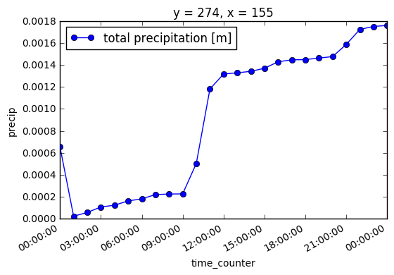
It is evident that the forecast precipitation is a cumulative value.
The hourly precipitation amount (in \(\frac{m}{hr}\)) is the hour-to-hour differences of the total precipitation values. To convert that to precipitation flux the factor is:
So, working backward from the end of the forecast period, we calculate the flux for each hour:
In [9]:
for hr in range(24, 1, -1):
    ds.precip.values[hr] = (ds.precip.values[hr] - ds.precip.values[hr-1]) / 3.6
    print(hr, ds.precip.values[hr, y, x])
24 2.53478194483e-06
23 7.41960118628e-06
22 3.80719171113e-05
21 3.07586419189e-05
20 3.72315601756e-06
19 3.96086963721e-06
18 5.9035503202e-07
17 4.94063392075e-06
16 1.63548651876e-05
15 7.79322969417e-06
14 3.79420170147e-06
13 3.09635652229e-06
12 3.78012191504e-05
11 0.000188606726523
10 7.70576459925e-05
9 3.61938469319e-07
8 1.35291985417e-06
7 1.09993359527e-05
6 5.07865479449e-06
5 1.09111574097e-05
4 4.44664894733e-06
3 1.38603910374e-05
2 9.56290983191e-06
The hour 1 flux is the hour 1 cumulative value divided by 3.6 because the cumulative value at hour 0 is, by definition, zero:
In [10]:
ds.precip.values[1] /= 36
print(1, ds.precip.values[1, y, x])
1 5.98205941868e-07
As above, we avoid restart artifacts from the HRDPS product by calculating the hour 0 flux from the difference between the cumulative precipitation values in the final 2 hours of the previous day’s forecast files:
In [11]:
day_m1_precip = {}
for hr in (23, 24):
    nc_filepath = gunzip_dir/'2016102500_0{}_2.5km_534x684.nc'.format(hr)
    with xarray.open_dataset(nc_filepath.as_posix()) as hr_ds:
        day_m1_precip[hr] = hr_ds.precip.values[0, ...]
ds.precip.values[0] = (day_m1_precip[24] - day_m1_precip[23]) / 36
print(0, ds.precip.values[0, y, x])
0 2.44207007604e-07
Finally, we update the metadata attributes of the precip variable to
reflect the change from cumulative to flux values:
In [12]:
ds.precip.attrs['units'] = 'kg m-2 s-1'
ds.precip.attrs['long_name'] = 'precipitation flux'
ds.precip.attrs['valid_max'] = 3
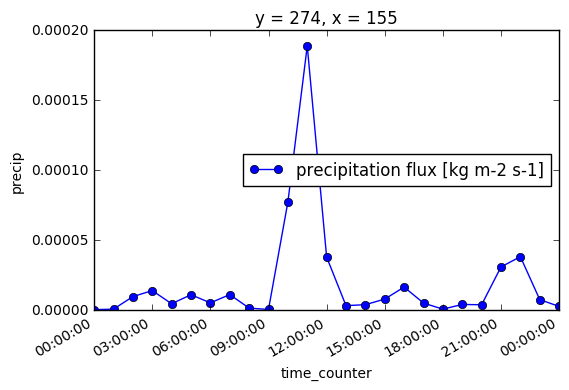
With that our precipitation near YQI now looks like:
In [13]:
ds.precip[:, y, x].plot(
    marker='o', label='{0.long_name} [{0.units}]'.format(ds.precip))
lgd = plt.legend(loc='best')
Calculation of solid precipitation component
NEMO uses the solid phase precipitation (snow) flux in addition to the total precipitation flux. Since the HRDPS product provides only total precipitation (which we have converted to flux above), we will calculate the snow flux by assuming that precipitation at grid points where the air temperature is >273.15 Kelvin is snow.
In [14]:
snow = ds.precip.copy()
snow.name = 'snow'
snow.attrs['short_name'] = 'snow'
snow.attrs['long_name'] = 'solid precipitation flux'
snow.values[ds.tair.values >= 273.15] = 0
snow
Out[14]:
<xarray.DataArray 'snow' (time_counter: 25, y: 684, x: 534)>
array([[[  0.00000000e+00,   0.00000000e+00,   0.00000000e+00, ...,
           0.00000000e+00,   0.00000000e+00,   0.00000000e+00],
        [  0.00000000e+00,   0.00000000e+00,   0.00000000e+00, ...,
           0.00000000e+00,   0.00000000e+00,   0.00000000e+00],
        [  0.00000000e+00,   0.00000000e+00,   0.00000000e+00, ...,
           0.00000000e+00,   0.00000000e+00,   0.00000000e+00],
        ...,
        [  0.00000000e+00,   0.00000000e+00,   0.00000000e+00, ...,
           0.00000000e+00,   0.00000000e+00,   0.00000000e+00],
        [  0.00000000e+00,   0.00000000e+00,   0.00000000e+00, ...,
           0.00000000e+00,   0.00000000e+00,   0.00000000e+00],
        [  0.00000000e+00,   0.00000000e+00,   0.00000000e+00, ...,
           0.00000000e+00,   0.00000000e+00,   0.00000000e+00]],

       [[  0.00000000e+00,   0.00000000e+00,   0.00000000e+00, ...,
           0.00000000e+00,   0.00000000e+00,   0.00000000e+00],
        [  0.00000000e+00,   0.00000000e+00,   0.00000000e+00, ...,
           0.00000000e+00,   0.00000000e+00,   0.00000000e+00],
        [  0.00000000e+00,   0.00000000e+00,   0.00000000e+00, ...,
           0.00000000e+00,   0.00000000e+00,   0.00000000e+00],
        ...,
        [  4.71105673e-10,   3.35895238e-10,   1.86492365e-10, ...,
           0.00000000e+00,   0.00000000e+00,   0.00000000e+00],
        [  4.66930149e-10,   3.34405960e-10,   1.79570322e-10, ...,
           0.00000000e+00,   0.00000000e+00,   0.00000000e+00],
        [  4.60884318e-10,   3.14873707e-10,   1.62259786e-10, ...,
           0.00000000e+00,   0.00000000e+00,   0.00000000e+00]],

       [[  0.00000000e+00,   0.00000000e+00,   0.00000000e+00, ...,
           0.00000000e+00,   0.00000000e+00,   0.00000000e+00],
        [  0.00000000e+00,   0.00000000e+00,   0.00000000e+00, ...,
           0.00000000e+00,   0.00000000e+00,   0.00000000e+00],
        [  0.00000000e+00,   0.00000000e+00,   0.00000000e+00, ...,
           0.00000000e+00,   0.00000000e+00,   0.00000000e+00],
        ...,
        [  0.00000000e+00,   0.00000000e+00,   0.00000000e+00, ...,
           0.00000000e+00,   0.00000000e+00,   0.00000000e+00],
        [  0.00000000e+00,   0.00000000e+00,   0.00000000e+00, ...,
           0.00000000e+00,   0.00000000e+00,   0.00000000e+00],
        [  0.00000000e+00,   0.00000000e+00,   0.00000000e+00, ...,
           0.00000000e+00,   0.00000000e+00,   0.00000000e+00]],

       ...,
       [[  0.00000000e+00,   0.00000000e+00,   0.00000000e+00, ...,
           0.00000000e+00,   0.00000000e+00,   0.00000000e+00],
        [  0.00000000e+00,   0.00000000e+00,   0.00000000e+00, ...,
           0.00000000e+00,   0.00000000e+00,   0.00000000e+00],
        [  0.00000000e+00,   0.00000000e+00,   0.00000000e+00, ...,
           0.00000000e+00,   0.00000000e+00,   0.00000000e+00],
        ...,
        [  8.63036891e-08,   4.41076745e-08,   1.20501846e-08, ...,
           0.00000000e+00,   0.00000000e+00,   0.00000000e+00],
        [  6.95294449e-08,   3.00454644e-08,   7.77361731e-09, ...,
           0.00000000e+00,   0.00000000e+00,   0.00000000e+00],
        [  4.83119125e-08,   2.01756123e-08,   6.08449439e-09, ...,
           0.00000000e+00,   0.00000000e+00,   0.00000000e+00]],

       [[  0.00000000e+00,   0.00000000e+00,   0.00000000e+00, ...,
           0.00000000e+00,   0.00000000e+00,   0.00000000e+00],
        [  0.00000000e+00,   0.00000000e+00,   0.00000000e+00, ...,
           0.00000000e+00,   0.00000000e+00,   0.00000000e+00],
        [  0.00000000e+00,   0.00000000e+00,   0.00000000e+00, ...,
           0.00000000e+00,   0.00000000e+00,   0.00000000e+00],
        ...,
        [  1.90385521e-07,   1.24513437e-07,   6.79671233e-08, ...,
           0.00000000e+00,   0.00000000e+00,   0.00000000e+00],
        [  1.85208925e-07,   1.17347238e-07,   6.19586229e-08, ...,
           0.00000000e+00,   0.00000000e+00,   0.00000000e+00],
        [  1.67548953e-07,   1.08436949e-07,   6.12702590e-08, ...,
           0.00000000e+00,   0.00000000e+00,   0.00000000e+00]],

       [[  0.00000000e+00,   0.00000000e+00,   0.00000000e+00, ...,
           0.00000000e+00,   0.00000000e+00,   0.00000000e+00],
        [  0.00000000e+00,   0.00000000e+00,   0.00000000e+00, ...,
           0.00000000e+00,   0.00000000e+00,   0.00000000e+00],
        [  0.00000000e+00,   0.00000000e+00,   0.00000000e+00, ...,
           0.00000000e+00,   0.00000000e+00,   0.00000000e+00],
        ...,
        [  3.47586359e-07,   2.59830652e-07,   1.76381094e-07, ...,
           0.00000000e+00,   0.00000000e+00,   0.00000000e+00],
        [  3.47946904e-07,   2.53843366e-07,   1.63869116e-07, ...,
           0.00000000e+00,   0.00000000e+00,   0.00000000e+00],
        [  3.07654394e-07,   2.29752730e-07,   1.54432540e-07, ...,
           0.00000000e+00,   0.00000000e+00,   0.00000000e+00]]])
Coordinates:
  * y             (y) int64 0 1 2 3 4 5 6 7 8 9 10 11 12 13 14 15 16 17 18 ...
  * x             (x) int64 0 1 2 3 4 5 6 7 8 9 10 11 12 13 14 15 16 17 18 ...
  * time_counter  (time_counter) datetime64[ns] 2016-10-26 ...
Attributes:
    units: kg m-2 s-1
    valid_min: 0.0
    valid_max: 3
    long_name: solid precipitation flux
    short_name: snow
    online_operation: inst(only(x))
    axis: TYX
    savelog10: 0.0
Merging the snow DataArray into the dataset to produce a new
DataSet object:
In [15]:
ds_with_snow = xarray.merge((ds, snow))
ds_with_snow
Out[15]:
<xarray.Dataset>
Dimensions:       (time_counter: 25, x: 534, y: 684)
Coordinates:
  * y             (y) int64 0 1 2 3 4 5 6 7 8 9 10 11 12 13 14 15 16 17 18 ...
  * x             (x) int64 0 1 2 3 4 5 6 7 8 9 10 11 12 13 14 15 16 17 18 ...
  * time_counter  (time_counter) datetime64[ns] 2016-10-26 ...
Data variables:
    tair          (time_counter, y, x) float64 279.8 279.5 279.2 279.9 279.7 ...
    seapres       (time_counter, y, x) float64 1.027e+05 1.027e+05 1.027e+05 ...
    precip        (time_counter, y, x) float64 0.0 0.0 0.0 0.0 0.0 0.0 0.0 ...
    nav_lon       (time_counter, y, x) float32 285.263 285.289 285.314 ...
    nav_lat       (time_counter, y, x) float32 40.6528 40.6412 40.6295 ...
    solar         (time_counter, y, x) float64 0.0 0.0 0.0 0.0 0.0 0.0 0.0 ...
    therm_rad     (time_counter, y, x) float64 244.5 244.3 243.9 244.5 243.9 ...
    v_wind        (time_counter, y, x) float64 -2.484 -2.443 -2.443 -2.67 ...
    u_wind        (time_counter, y, x) float64 1.914 1.888 1.881 2.001 1.927 ...
    qair          (time_counter, y, x) float64 0.002977 0.002969 0.003103 ...
    snow          (time_counter, y, x) float64 0.0 0.0 0.0 0.0 0.0 0.0 0.0 ...
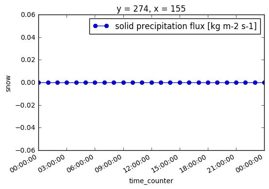
Although we can see above that there are non-zero snow fluxes at some grid points it appears that there is no significant snow flux at YQI on 2016-10-26:
In [16]:
ds_with_snow.snow[:, y, x].plot(
    marker='o', label='{0.long_name} [{0.units}]'.format(ds_with_snow.snow))
lgd = plt.legend(loc='best')
Storing the atmospheric forcing file
The forcing files are stored as netCDF4/HDF5 files. Doing so allows Lempel-Ziv deflation to be applied to each of the variables, resulting in a 50% to 80% reduction in the file size on disk.
The time units must also be specified when storing the file. We will use
the fairly common seconds since 1970-01-01 00:00:00 units.
Those things are applied to the dataset by providing an
encoding dict:
In [17]:
encoding = {var: {'zlib': True} for var in ds_with_snow.data_vars}
encoding['time_counter'] = {
    'units': 'seconds since 1970-01-01 00:00:00',
    'zlib': True,
}

encoding
Out[17]:
{'nav_lat': {'zlib': True},
 'nav_lon': {'zlib': True},
 'precip': {'zlib': True},
 'qair': {'zlib': True},
 'seapres': {'zlib': True},
 'snow': {'zlib': True},
 'solar': {'zlib': True},
 'tair': {'zlib': True},
 'therm_rad': {'zlib': True},
 'time_counter': {'units': 'seconds since 1970-01-01 00:00:00', 'zlib': True},
 'u_wind': {'zlib': True},
 'v_wind': {'zlib': True}}
And, with that, we can store the dataset on disk:
In [18]:
ds_with_snow.to_netcdf('gem2.5_y2016m10d26.nc', encoding=encoding)
It is at this point that the concatenation of the hourly forecast files
into the forcing dataset occurs, as well as the calculation on the
precipitation variable. The to_netcdf() method may take 60 seconds
or longer, depending on the memory size, CPU speed, and number of cores
available.
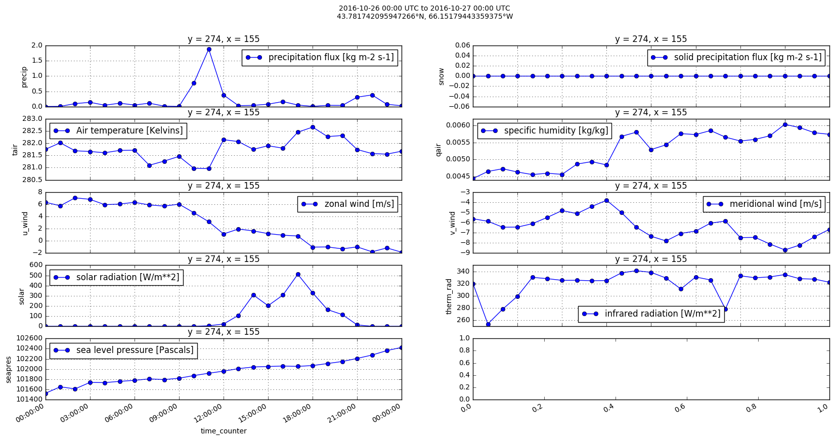
Plots of forcing variables time-series at a point
In [19]:
fig, axs = plt.subplots(5, 2, figsize=(20, 10))
var_axs = [
    ('precip', 0, 0),
    ('snow', 0, 1),
    ('tair', 1, 0),
    ('qair', 1, 1),
    ('u_wind', 2, 0),
    ('v_wind', 2, 1),
    ('solar', 3, 0),
    ('therm_rad', 3, 1),
    ('seapres', 4, 0),
]
for var, ax_row, ax_col in var_axs:
    factor = 10000 if var == 'precip' else 1
    (ds_with_snow.data_vars[var][:, y, x] * factor).plot(
        ax=axs[ax_row, ax_col], marker='o',
        label='{0.long_name} [{0.units}]'.format(ds_with_snow.data_vars[var]))
    axs[ax_row, ax_col].legend(loc='best')
    axs[ax_row, ax_col].grid()
fig_title = fig.suptitle(
    '{0[0]:%Y-%m-%d %H:%M} UTC to {0[24]:%Y-%m-%d %H:%M} UTC\n'
    '{1}°N, {2}°W'
    .format(
        pandas.to_datetime(ds_with_snow.time_counter.values),
        ds_with_snow.nav_lat[0, y, x].values,
        abs(ds_with_snow.nav_lon[0, y, x].values - 360),
))
In [20]:
ds.close()
ds_with_snow.close()